Tutorial 2.: Running an Example Analysis in mesalab with Google Colab
This tutorial will guide you through running a full mesalab analysis
within a Google Colab environment. We’ll set up mesalab, process a
sample of real MESA data to identify specific stellar phenomena, and
inspect the results.
The provided example data allows you to test mesalab’s core
functionality for filtering MESA outputs without needing to install
the MESA SDK, GYRE, or RSP.
Note
The full tutorial is available at the following Colab link:
Prerequisites
An active Google account (for Colab access).
1. Set up mesalab and Get Example Data
1.1 Clone the mesalab repository
First, clone the mesalab repository from GitHub. This will give you
access to the source code and the example/ directory containing the
sample MESA data and configuration files.
💡 Note: This step is a one-time operation per session. If you’ve already run this cell, you can skip it.
!git clone https://github.com/konkolyseismolab/mesalab
Upon successful connection and cloning, you will see something similar:
Cloning into 'mesalab'...
remote: Enumerating objects: 17007, done.
remote: Counting objects: 100% (1256/1256), done.
remote: Compressing objects: 100% (348/348), done.
remote: Total 17007 (delta 618), reused 1155 (delta 529), pack-reused 15751 (from 2)
Receiving objects: 100% (17007/17007), 861.96 MiB | 22.93 MiB/s, done.
Resolving deltas: 100% (8864/8864), done.
Updating files: 100% (929/929), done.
1.2 Install mesalab and its dependencies
Now, install mesalab and all its required Python packages.
💡 Note: This step is a one-time operation per session. If you’ve already run this cell, you can skip it.
# Navigate in the main directory
%cd mesalab

# Install the package
!pip install -e .
Upon successfull installation, you will see something similar:
Obtaining file:///content/mesalab
  Installing build dependencies ... done
  Checking if build backend supports build_editable ... done
  Getting requirements to build editable ... done
  Preparing editable metadata (pyproject.toml) ... done
  ...
(Check dependencies)
  ...
Building wheels for collected packages: mesalab
  Building editable for mesalab (pyproject.toml) ... done
  Created wheel for mesalab: filename=mesalab-2.2.0.editable-py3-none-any.whl size=4567 sha256=4743ff9c2aa1d4dfe9976940b9330515421f82c261cd1c4487a2faab7463d1b4
  Stored in directory: /tmp/pip-ephem-wheel-cache-3_j9zmho/wheels/63/36/82/a810ed5c505fd0aa9429ceb5fa4bdd5aec5db1b8aa04ffb789
Successfully built mesalab
Installing collected packages: mesalab
  Attempting uninstall: mesalab
    Found existing installation: mesalab 2.2.0.
    Uninstalling mesalab-2.2.0.
      Successfully uninstalled mesalab-2.2.0.
Successfully installed mesalab-2.2.0.
2. Examine the Example Data and Configuration
Once you have successfully installed the package, navigate to the
example/ directory within mesalab/.
%cd example/
This directory contains two pre-defined datasets. In this tutorial, we
will focus on the MESA_grid dataset, which consists of real stellar
evolution outputs from MESA. It is designed to demonstrate
mesalab’s core blue loop filtering and analysis capabilities.
2.1. Dataset Overview
Grid Parameters: The dataset includes a 2x2 grid of models with masses of 4 and 5 M⊙ and metallicities (Z) of 0.0090 and 0.0100.
Evolutionary Coverage: The simulations cover stellar evolution from the pre-main sequence (pre-MS) to a point after the blue loop phase.
Key Feature: A defining characteristic of this dataset is the differing blue loop behavior: models with 5 M⊙ exhibit blue loop crossings, while models with 4 M⊙ do not.
This example dataset is located in the example/MESA_grid directory.
The corresponding example_MESA_base.yaml configuration file is set
up to identify blue loop crossers and generate plots. It also prepares
filtered output files, which can be used as input for a subsequent GYRE
workflow.
3. Run the MESA_grid Example
You can easily run your first example by executing mesalab with the
provided configuration file:
! mesalab --config example_MESA_base.yaml
================================================================================
                    mesalab CLI - Starting Analysis Workflow
                                Version: 2.2.0
================================================================================

2026-06-02 15:09:04,785 - WARNING: PyMultiNest not imported.  MultiNest fits will not work.

======================================================================
    Starting MESA Analysis Workflow...
======================================================================

Performing MESA Run Analysis: 100% 4/4 [00:01<00:00,  3.05it/s]

======================================================================
    MESA Analysis Workflow Completed Successfully.
======================================================================


======================================================================
    MESA RSP workflow is disabled in configuration.
======================================================================


======================================================================
    Starting Plotting Workflow...
======================================================================


======================================================================
Full Instability Strip Crossings Matrix (for Heatmap):
======================================================================
        4.0  5.0
initial_Z
0.009      0.0  2.0
0.010      0.0  2.0
======================================================================

Calculating BCs serially: 100% 373/373 [00:01<00:00, 239.75it/s]
2026-06-02 15:09:12,549 - WARNING: No valid CMD plots for combined data after dropping NaNs in G_BP_minus_G_RP or M_G.

======================================================================
    Plotting Workflow Completed Successfully.
======================================================================


======================================================================
    GYRE workflow is disabled in configuration.
======================================================================


================================================================================
║                  mesalab Workflow Finished Successfully!                    ║
================================================================================
3.1. Checking the Ouput
Note
⚠️ IMPORTANT: The CMD (Color-Magnitude Diagram) is NOT generated in Google Colab.
Due to dependency limitations and incomplete isochrones compatibility in the Colab environment, the pipeline cannot reliably construct Gaia-based photometric transformations.
As a result, the CMD step is automatically skipped even in a successful run.
Instead, the analysis focuses on HR-diagram-based evolutionary tracking and internal stellar parameters.
After a successful run, you will find the generated plots in the
example/MESA_grid_base_output/plots directory. Here are some
examples of the plots generated for this grid:
>>> from IPython.display import Image
>>> Image(filename='MESA_grid_base_output/plots/HRD_all_blue_loop_data.png')
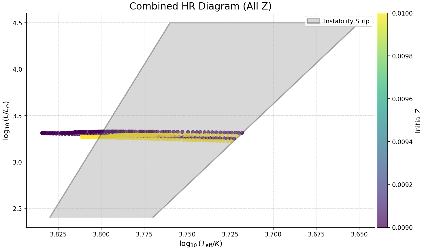
Figure 1: Gaia Color-Magnitude Diagram (CMD) for the 5 Msun models that undergo blue loop evolution. This plot specifically focuses on models that are currently within the blue loop phase and have crossed the red (cool) boundary of the Instability Strip (IS), indicating evolutionary stages relevant for pulsating stars.
>>> Image(filename='MESA_grid_base_output/plots/mesa_grid_blue_loop_heatmap.png')
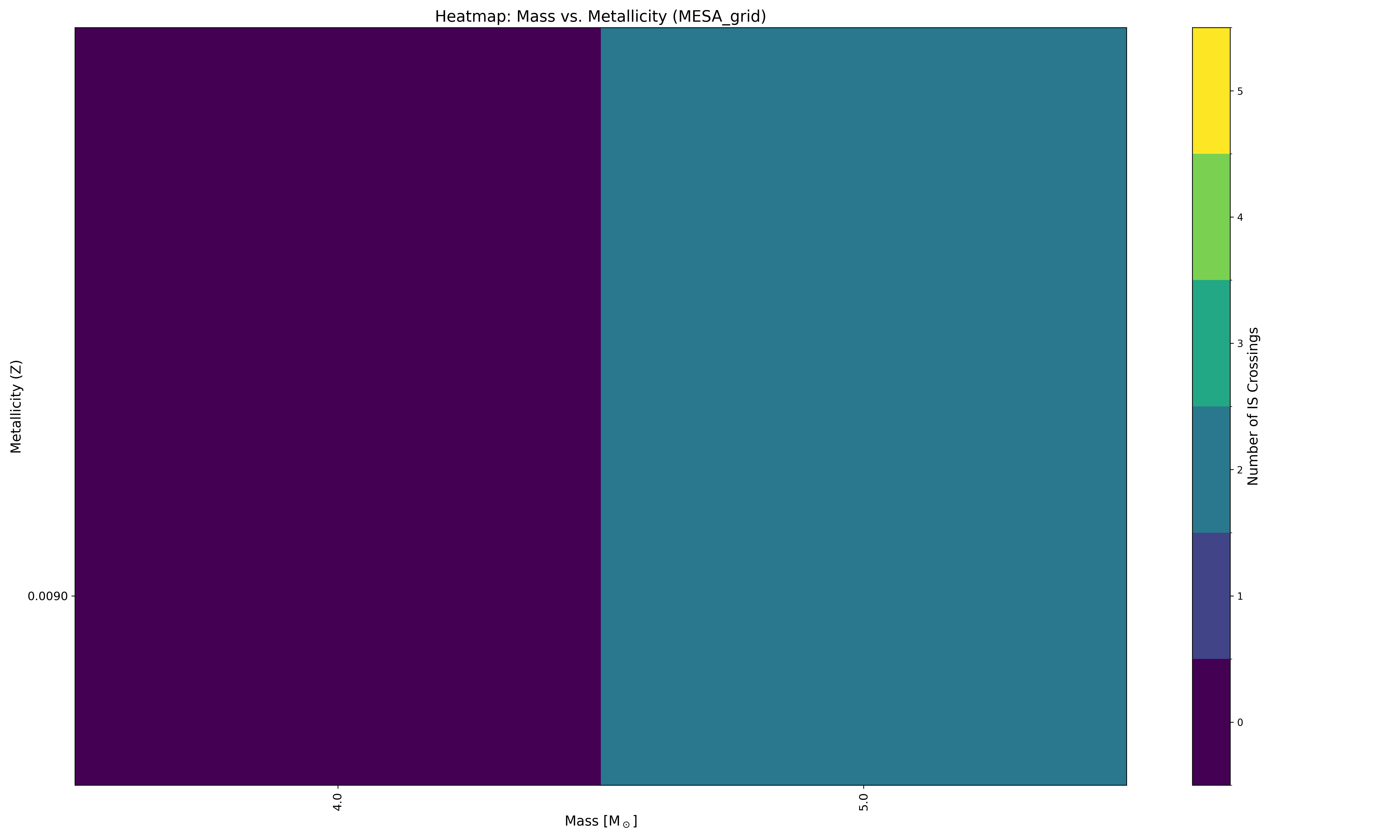
Figure 2: Heatmap visualizing the number of instability strip crossings for different initial masses and metallicities.
3.2. Additional Plots and CSVs
You can find more plots and CSV files in the
example/MESA_grid_base_output/ directory. These include HR diagrams
for each metallicity and a color-magnitude diagram (CMD) of the blue
loop evolutionary tracks.