Tutorial 3: Running GYRE and RSP with mesalab: example/MESA_grid_gyre, example/MESA_grid_gyre
The base of the MESA_grid dataset is discussed in Tutorial 2. that demonstrates how the mesalab pipeline filters, processes, and prepares stellar evolution data for pulsation analysis.
Since pulsation analysis with GYRE or RSP requires the installation of MESA, MESASDK and GYRE it is challenging to set up and run interactively on a platform like Google Colab. Therefore, this tutorial walks through what the output of a successful run looks like utilizing GYRE and/or RSP workflow without an interacitve Google Colab notebook.
MESA Grid dataset
This set of runs are actual MESA stellar evolution outputs, providing standard profile, history, and inlist files for demonstrating the analysis.
Grid Structure & Parameters: It contains a 2x2 grid of models with initial masses of 4 and 5 solar masses and metallicities (Z) of 0.0090 and 0.0100.
Evolutionary Coverage: Simulations cover stellar evolution from the pre-main sequence (pre-MS) through to after the blue loop phase.
Blue Loop Behavior: A key feature is the differing blue loop behavior: 5 Msun models exhibit blue loop crossings, while 4 Msun models do not. This highlights mesalab’s capability to identify and filter profiles based on evolutionary characteristics.
Location: These models are found in the
example/MESA_griddirectory.YAML Configuration Files: The corresponding
example_MESA_gyre.yamlandexample_MESA_rsp.yamlconfiguration files set up is responsible to identify blue loops, generate plots, and run GYRE or RSP on the relevant stellar profiles.
Run MESA grid example with GYRE
You can easily run your first example by executing mesalab with the provided configuration file:
$ mesalab --config example/example_MESA_gyre.yaml
Upon execution, you’ll see terminal output featuring a live-updating progress bar followed by a structured final workflow summary:
================================================================================
                   mesalab CLI - Starting Analysis Workflow
                              Version: 2.2.0
================================================================================

======================================================================
    Starting MESA Analysis Workflow...
======================================================================

Performing MESA Run Analysis: 100%|███████████████████████████████████| 4/4 [00:03<00:00,  1.15it/s]

======================================================================
    MESA Analysis Workflow Completed Successfully.
======================================================================

======================================================================
    Starting Plotting Workflow...
======================================================================

======================================================================
    Full Instability Strip Crossings Matrix (for Heatmap):
======================================================================
            4.0  5.0
initial_Z
0.009       0.0  2.0
0.010       0.0  2.0
======================================================================

Calculating BCs serially: 100%|█████████████████████████████████████████████| 373/373 [00:04<00:00, 88.77it/s]

======================================================================
    Plotting Workflow Completed Successfully.
======================================================================

======================================================================
    Starting GYRE Workflow...
======================================================================

[2026-06-02 01:04:30] GYRE Pipeline: Initializing GYRE workflow from mesalab configuration...
GYRE Pipeline Workflow: 100%|██████████████████████████████████████████| 30/30 [00:45<00:00,  1.50s/it]

--- GYRE Pipeline Workflow Summary ---
Total runs: 30
Successful runs: 30
Failed runs: 0
--------------------------------------
Final workflow statistics saved to: example/MESA_grid_output/gyre_outputs/gyre_workflow_summary.json

[2026-06-02 01:05:15] GYRE Pipeline: All individual GYRE runs completed successfully.

======================================================================
    GYRE Workflow Completed Successfully.
======================================================================

================================================================================
║                  mesalab Workflow Finished Successfully!                     ║
================================================================================
After the workflow completes, you will find the generated plots in the example/MESA_grid_output/plots directory. Here are some examples of the plots generated for this grid:
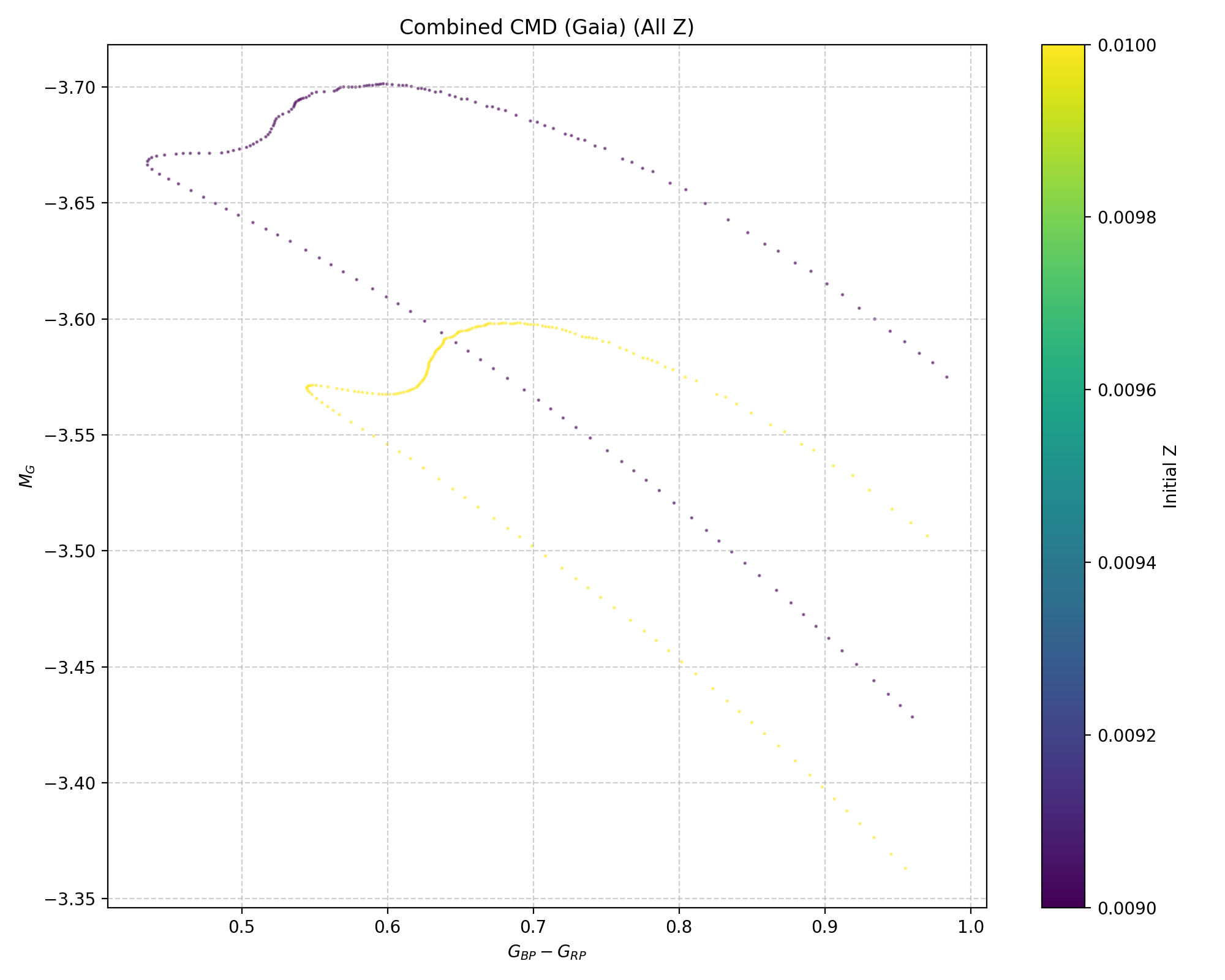
Gaia Color-Magnitude Diagram (CMD) for the 5 Msun models that undergo blue loop evolution. This plot specifically focuses on models that are currently within the blue loop phase and have crossed the red (cool) boundary of the Instability Strip (IS), indicating evolutionary stages relevant for pulsating stars.
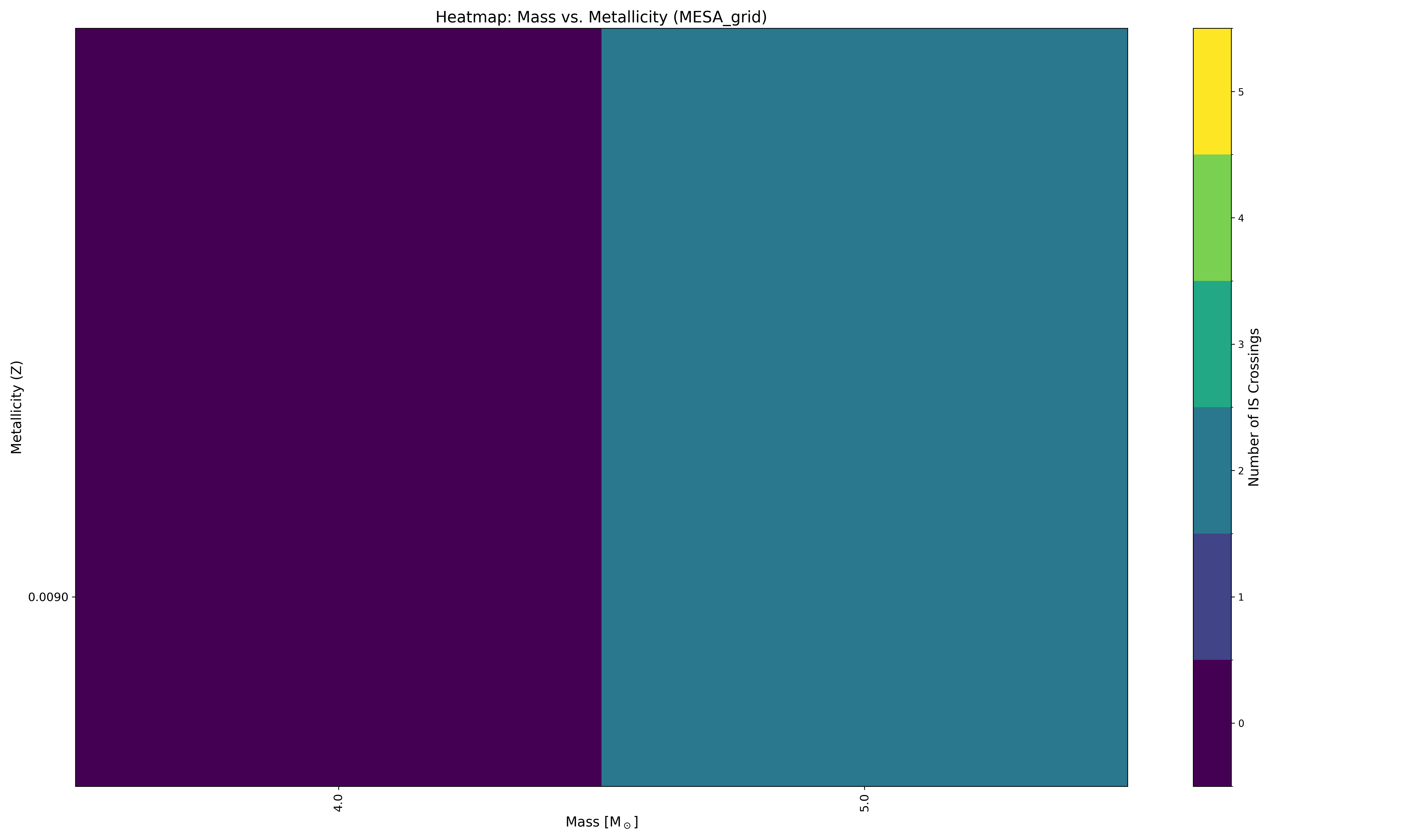
Heatmap visualizing the number of instability strip crossings for different initial masses and metallicities.
Understanding GYRE Output
After the GYRE workflow is complete, a structured output directory is created to store the run data. To prevent data loss during long grid runs, mesalab serializes progress metrics in real time.
The main output folder is gyre_outputs. At its root, a live-updated summary file is maintained, followed by separate subdirectories for each MESA stellar model run:
example/MESA_grid_output/
└── gyre_output/
    ├── gyre_workflow_summary.json        # Live-updating global runtime summary
    └── run_5.0MSUN_z0.0090/
         └── profile00018
             ├── summary.h5
             └── detail.l<l>.n<n>.TXT  # Multiple detail files, one per mode
This profile00018 directory contains:
summary.h5: This is a binary HDF5 file containing an overview of all calculated pulsation modes for a specific stellar profile. It’s data should look like this:E_norm eta freq l n_g n_p n_pg omega ---------------------- --- ----------------------- --- --- --- ---- ----------------------- 7.716313969427929e-06 0.0 (0.3288290815023021+0j) 0 0 2 2 (4.1285738058857735+0j) 4.977767116023725e-06 0.0 (0.4253575871382588+0j) 0 0 3 3 (5.340525796473679+0j) 3.5467134221115035e-06 0.0 (0.5281812006857637+0j) 0 0 4 4 (6.631515253912462+0j) 2.8337113271118767e-06 0.0 (0.635019445275698+0j) 0 0 5 5 (7.972909926383766+0j) 2.4590763873617003e-06 0.0 (0.7390031628616821+0j) 0 0 6 6 (9.278464929921713+0j) 2.6585877070418085e-06 0.0 (0.8449905263159454+0j) 0 0 7 7 (10.609176467091832+0j) 3.5417203213359843e-06 0.0 (0.9541649016993462+0j) 0 0 8 8 (11.979902147504905+0j) 4.947878175758324e-06 0.0 (1.0683611742967478+0j) 0 0 9 9 (13.413679651676546+0j) 7.228378461640029e-06 0.0 (1.1830569761877034+0j) 0 0 10 10 (14.853728935543636+0j)
detail.l<l>.n<n>.TXT: These are plain text files, each containing detailed information about the eigenfunction (e.g., displacement, velocity, luminosity perturbations) of a specific pulsation mode in the star’s interior. The filename indicates the spherical harmonic degree (l) and the radial order (n). For example, inspecting adetail.l0.n+10.TXTfile (for a 5 Msun, Z=0.0100 model at a specific evolutionary stage) you should see:Gamma_1 P T dW_dx ... rho x xi_h xi_r ----------------- --------------------- ----------------- ----- ... --------------------- --------------------- ---- --------------------------- 1.606969163191305 4.521157801068377e+19 147308873.3222435 0.0 ... 5315.50896647388 0.0 0j 0j 1.606971014744742 4.520751437574627e+19 147304132.5888782 0.0 ... 5315.215595668408 1.208472088924861e-05 0j (-2.981450615162198e-08+0j) 1.606972222965719 4.520489787509158e+19 147301039.0453129 0.0 ... 5315.024158263152 1.522589262621941e-05 0j (-3.756430947851294e-08+0j) 1.606974103631016 4.520082534000535e+19 147296223.7726631 0.0 ... 5314.726179017575 1.918363197076153e-05 0j (-4.73289618981165e-08+0j) # ... (approximately 1240 more rows) ... 1.476818050225248 1131.83485879053 6028.82736586096 -0.0 ... 2.834199661473333e-09 0.9999996951714716 0j (371.9168322490516+0j) 1.476826592953945 1131.761019649602 6028.778110862875 -0.0 ... 2.834038079040092e-09 0.9999998013548269 0j (371.9271310542792+0j) 1.476830863819082 1131.724100088799 6028.753484881346 -0.0 ... 2.833957286079444e-09 0.999999854448763 0j (371.9322807595553+0j) 1.476835134309931 1131.687180535459 6028.728860071846 -0.0 ... 2.833876491880485e-09 0.999999907544212 0j (371.9374306673092+0j) 1.476837724407599 1131.664786712097 6028.713924351446 -0.0 ... 2.833827484927481e-09 0.999999939750376 0j (371.9405544796087+0j) 1.476839019409059 1131.653589801338 6028.706456636452 -0.0 ... 2.833802981287909e-09 0.9999999558536716 0j (371.9421164141642+0j) 1.476840314376306 1131.642392891255 6028.698989028436 -0.0 ... 2.833778477534831e-09 0.9999999719571027 0j (371.9436783669861+0j) 1.476841158114899 1131.635097354881 6028.694123442688 -0.0 ... 2.833762511636029e-09 0.9999999824496407 0j (371.9446960938195+0j) 1.476842001837285 1131.627801818827 6028.689257907953 -0.0 ... 2.833746545684138e-09 0.9999999929422394 0j (371.9457138287099+0j)
Tip
You can access the data of GYRE output files using various tools. For Python users, the pygyre library is one of the most convenient options.
For instance, to load the summary.h5 file shown above into a Python object, you would use:
>>> import pygyre
>>> import numpy
>>> s = pygyre.read_output('example/MESA_grid_output/run_5.0MSUN_z0.0100/profile00030/summary.h5')
>>> print(s)
Run MESA grid example with RSP
Similar to the case of GYRE, you can easily run your first example by executing mesalab with the provided configuration file:
$ mesalab --config example/example_MESA_rsp.yaml
Upon successful execution, you’ll see a clean, modern progress interface followed by a unified performance matrix:
================================================================================
                    mesalab CLI - Starting Analysis Workflow
                              Version: 2.2.0
================================================================================


======================================================================
        Starting MESA Analysis Workflow...
======================================================================

Performing MESA Run Analysis: 100%|██████████████████████████████████████████████████████████████████| 4/4 [00:03<00:00,  1.25it/s]

======================================================================
        MESA Analysis Workflow Completed Successfully.
======================================================================


======================================================================
        Starting MESA RSP Workflow...
======================================================================

MESA RSP Workflow: 100%|█████████████████████████████████████████████████████████████████████████████| 373/373 [1:45:53<00:00, 17.03s/it]

--- MESA RSP Workflow Summary ---
Total runs: 373
Successful runs: 373
Failed runs: 0
Timed out runs: 0
Runs with unexpected errors: 0
---------------------------------
Final workflow statistics saved to: example/MESA_grid_output/rsp_outputs/rsp_workflow_summary.json

======================================================================
        MESA RSP Workflow Completed.
======================================================================


======================================================================
        Plotting workflow is disabled in configuration.
======================================================================


======================================================================
        GYRE workflow is disabled in configuration.
======================================================================


================================================================================
║                   mesalab Workflow Finished Successfully!                    ║
================================================================================
Understanding RSP Output
After the RSP workflow completes, a dedicated rsp_outputs directory is created. Similar to the GYRE layer, progress tracking is handled through real-time state serialization, writing states directly to disk as each model completes to buffer against server interrupts or unexpected runtime timeouts.
The typical directory tree layout within the output workspace now explicitly lists the global intermediate stats file:
example/MESA_grid_output/
└── rsp_outputs/
    ├── rsp_workflow_summary.json          # Live-updating global runtime summary
    ├── run_5.0MSUN_z0.0090/
    │   ├── model2073
    │   │   ├── LOGS
    │   │   │    ├── LINA_eigen1.data
    │   │   │    ├── LINA_work1.data
    │   │   │    ├── LINA_period_growth.data
    │   │   │    ├── history.data
    │   │   │    ├── profile1.data
    │   │   │    ├── profiles.index
    │   │   │    └── ... (additonal eigen and work data files)
    │   │   ├── photos
    │   │   │    ├── 1000
    │   │   │    └── x200
    │   │   ├── inlist_rsp
    │   │   └── rsp_final_M5.0Z0.0090Mod2073.mod
    │   └── ... (additional model directories as per the run)
    └── ... (additional run directories as per the run)
The LOGS directory contains:
LINA_eigen<mode>.data: These files contain radial displacement eigen functions for the given mode. E.g.,LINA_eigen1.data:ZONE TEMP. FRAC. RADIUS ABS(dR/R) PH(dR/R) ABS(dT/T) PH(dT/T) ABS(dL/L) PH(dL/L) ABS(dE_T) PH(dE_T) 0 150 2000080.00 0.123268 0.000163 -0.098954 0.001073 3.042632 0.001161 3.042569 0.000000e+00 0.000000 1 149 1799350.00 0.135102 0.000329 -0.098957 0.001489 3.042638 0.001737 3.042641 0.000000e+00 0.000000 2 148 1632500.00 0.146808 0.000503 -0.098958 0.001958 3.042638 0.002717 3.042654 0.000000e+00 0.000000 3 147 1491620.00 0.158447 0.000692 -0.098959 0.002492 3.042637 0.003975 3.042648 0.000000e+00 0.000000 4 146 1370180.00 0.170060 0.000899 -0.098959 0.003106 3.042636 0.005315 3.042862 0.000000e+00 0.000000 5 145 1263930.00 0.181673 0.001131 -0.098953 0.003816 3.042602 0.001271 -0.098325 0.374559e-11 -0.029433 # ... (140 more rows) ... 145 5 4526.44 0.995437 0.968194 -0.002383 1.503676 2.797751 3.256292 2.489870 3.835510e-09 -2.835612 146 4 4494.46 0.995788 0.970526 -0.002196 1.421361 2.780857 3.254585 2.490362 4.084549e-09 -2.839738 147 3 4467.79 0.996237 0.973556 -0.001958 1.352226 2.764817 3.252847 2.490869 4.290449e-09 -2.842108 148 2 4446.81 0.996863 0.977848 -0.001630 1.297338 2.750643 3.251079 2.491390 4.473423e-09 -2.843173 149 1 4428.19 1.000000 1.000000 0.000000 1.247333 2.737229 3.247400 2.492486 0.000000e+00 0.000000
LINA_work<mode>.data: These files contain differentian work data for the given mode. E.g.,LINA_work1.data:ZONE log(T) X WORK(P) WORK(P_NU) WORK(P_T) CWORK(P) CWORK(P_NU) CWORK(P_T) 0 150 0.63010480E+01 1.232682e-01 4.884869e-09 0.000000e+00 0.0 4.884869e-09 0.000000 0.0 1 149 0.62551146E+01 1.351016e-01 -3.828003e-09 0.000000e+00 0.0 1.056867e-09 0.000000 0.0 2 148 0.62128531E+01 1.468076e-01 -7.364953e-09 0.000000e+00 0.0 -6.308086e-09 0.000000 0.0 3 147 0.61736593E+01 1.584471e-01 -7.786172e-09 0.000000e+00 0.0 -1.409426e-08 0.000000 0.0 4 146 0.61367768E+01 1.700598e-01 -9.630502e-09 0.000000e+00 0.0 -2.372476e-08 0.000000 0.0 5 145 0.61017226E+01 1.816735e-01 1.493473e-06 -0.380027e-09 0.0 1.256225e-05 -3.800277e-09 0.0 # ... (140 more rows) ... 146 4 0.36526775E+01 9.957880e-01 3.633752e-06 -2.835302e-10 0.0 4.718881e-03 -0.009395 0.0 147 3 0.36500924E+01 9.962367e-01 3.601383e-06 -2.910590e-10 0.0 4.722482e-03 -0.009395 0.0 148 2 0.36480489E+01 9.968628e-01 3.589575e-06 -2.989903e-10 0.0 4.726072e-03 -0.009395 0.0 149 1 0.36462261E+01 1.000000e+00 7.324720e-06 0.000000e+00 0.0 4.733397e-03 -0.009395 0.0 150 #KINETIC ENERGY: 9.563258e+44 NaN NaN NaN NaN NaN NaN
LINA_period_growth.data: This file contains growth rate data for the selected modes.0 0.70242E+01 -0.47580E-02 1 0.48162E+01 -0.93693E-01 2 0.35122E+01 -0.20679E+00 3 0.27596E+01 -0.28529E+00 4 0.22537E+01 -0.31895E+00 5 0.18990E+01 -0.33536E+00 6 0.16387E+01 -0.37024E+00 7 0.14418E+01 -0.35532E+00 8 0.12860E+01 -0.22096E+00 9 0.12053E+01 -0.17340E+00 10 0.11399E+01 -0.46921E+00 11 0.10392E+01 -0.37776E+00 12 0.94880E+00 -0.39381E+00 13 0.87543E+00 -0.45720E+00 14 0.81750E+00 -0.47711E+00
profile1.data: This file contains the radial profile of the star in MESA format.profiles.index: This file connects the actual model number to the given profile file.rsp_final_M<mass>Z<metallicity>Mod<model_number>.mod: This file contains the final output model of the RSP output.